贝叶斯网络
Bayesian Network
Reference
Definition
- A Bayesian Network is a DAG (Directed Acyclic Graph) whose nodes represent the random variables \(X_1, \dots, X_n\)
- For each node \(X_i\) there is a CPD (Conditional Probablity Distribution) \(P(X_i | \text{Par}_G(X_i))\)
Meaning
The BN represent a joint distribution via the chain rule for Bayesian Networks \(P\left(X_{1}, \ldots, X_{n}\right)=\Pi_{i} P\left(X_{i} \mid \operatorname{Par}_{G}\left(X_{i}\right)\right)\)
Example
For example, we consider the following example where the random variables are discrete and model our belief of the relationship between the Difficulty of the course, Intelligence of the student, Grade the student receive, SAT score the student get, and Recommandation Letter the student get as the BN below:
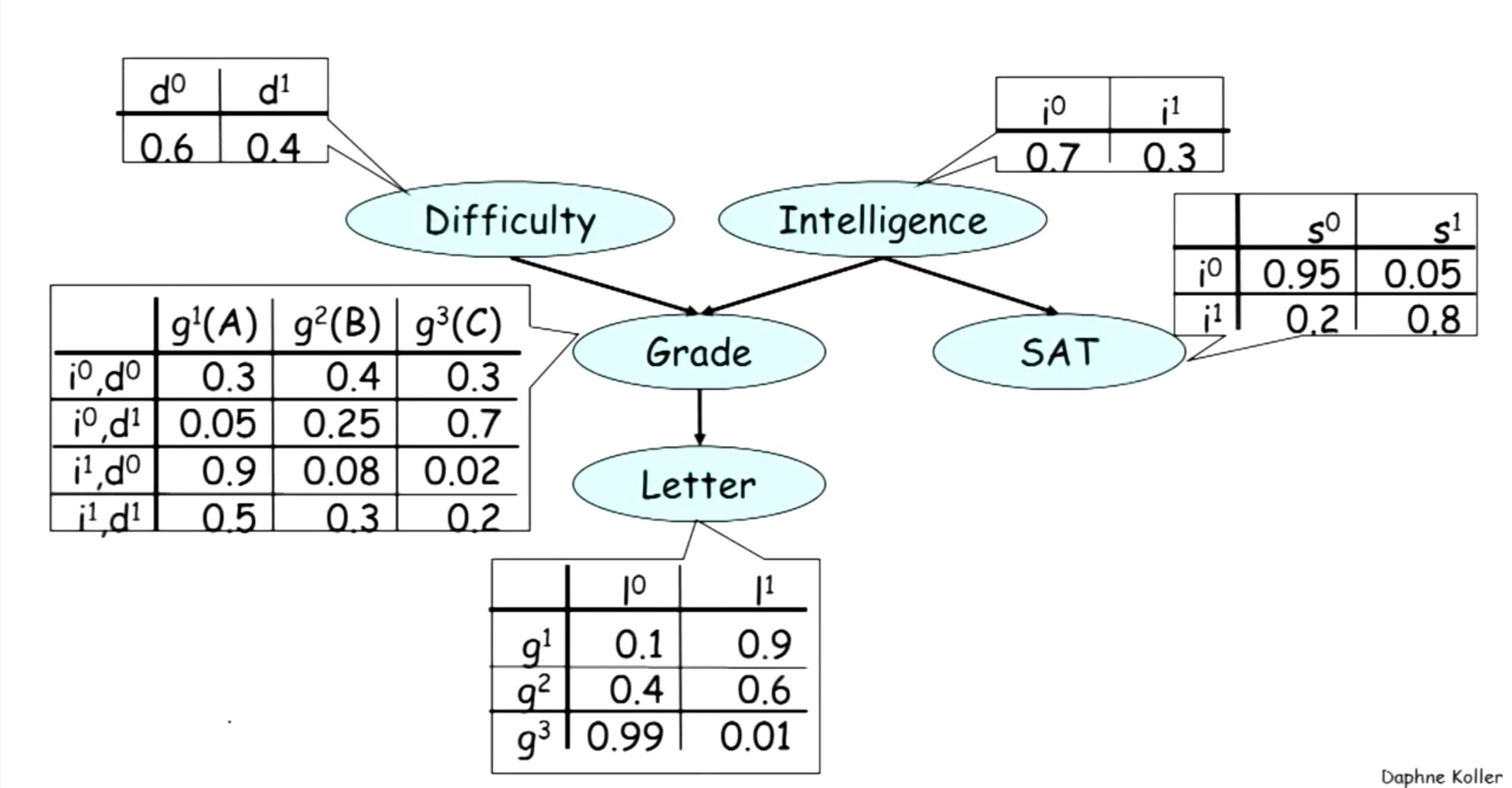
then the joint distribution of these random variables will be: \(P(D, I, G, S, L)=P(D) P(I) P(G \mid I, D) P(S \mid I) P(L \mid G)\)
Rigor
In order to see that BN is a legal distribution, we need some mathmatical rigor to show that BN representation of joint probability distribution satisfies the two vital properties:
- \[P \ge 0\]
- \[\sum P = 1\]
First, it’s obvious that the first property is true, since joint probability distribution is the product of CPDs, and given the CPDs are non-negative, we know that \(P \ge 0\) .
The second property is a little trickier to see, as it uses an important conditional probability summation trick: \(\begin{align*} \sum_{A, B} P(A, B)&=\sum_{A, B} P(A) P(B|A)\\ &=\sum_A \left(\sum_B P(A) P(B|A)\right)\\ &=\sum_A \left( P(A)\sum_B P(B|A)\right)\\ &=\sum_A P(A)\\ &=1 \end{align*}\) And in the above example, we can get same result using this trick: \(\begin{align*} \sum_{D,I,G,S,L} P(D,I,G,S,L) &= \sum_{D,I,G,S,L} P(D) P(I) P(G|I,D) P(S|I) P(L|G)\\ &= \sum_{D,I,G,S} P(D) P(I) P(G|I,D) P(S|I) \sum_L P(L|G)\\ &= \sum_{D,I,G,S} P(D) P(I) P(G|I,D) P(S|I)\\ &= \sum_{D,I,G} P(D) P(I) P(G|I,D) \sum_S P(S|I)\\ &= \sum_{D,I} P(D) P(I) \sum_G P(G|I,D)\\ &= \sum_{D,I} P(D) P(I)\\ &= \sum_{D} P(D) \sum_I P(I)\\ &= 1 \end{align*}\) so the BN representation of joint probability is a legal distribution.
Flow of Probabilistic Influence
The question here is when can X influence Y ? By influence, we mean condition on X will change belief about Y.
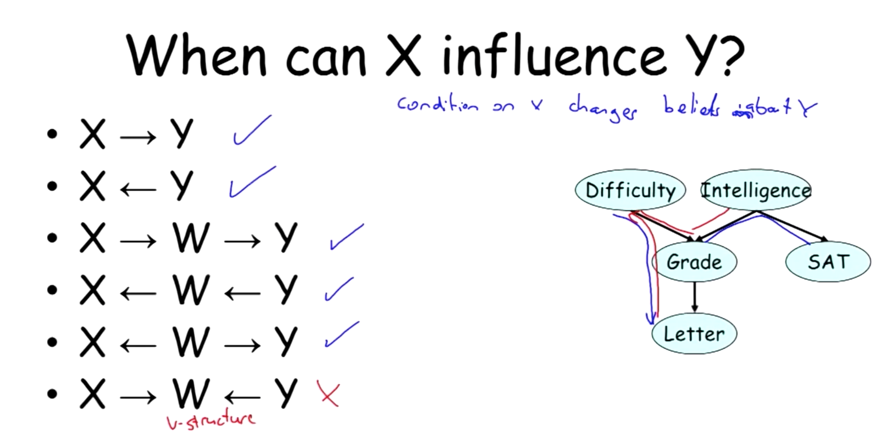
It turns out \(X_1\) can influence \(X_n\) if the trails \(X_1 - \ldots - X_n\) along them is active which means that it has no v-structures like \(X_{i - 1} \rightarrow X_{i} \leftarrow X_{i + 1}\).
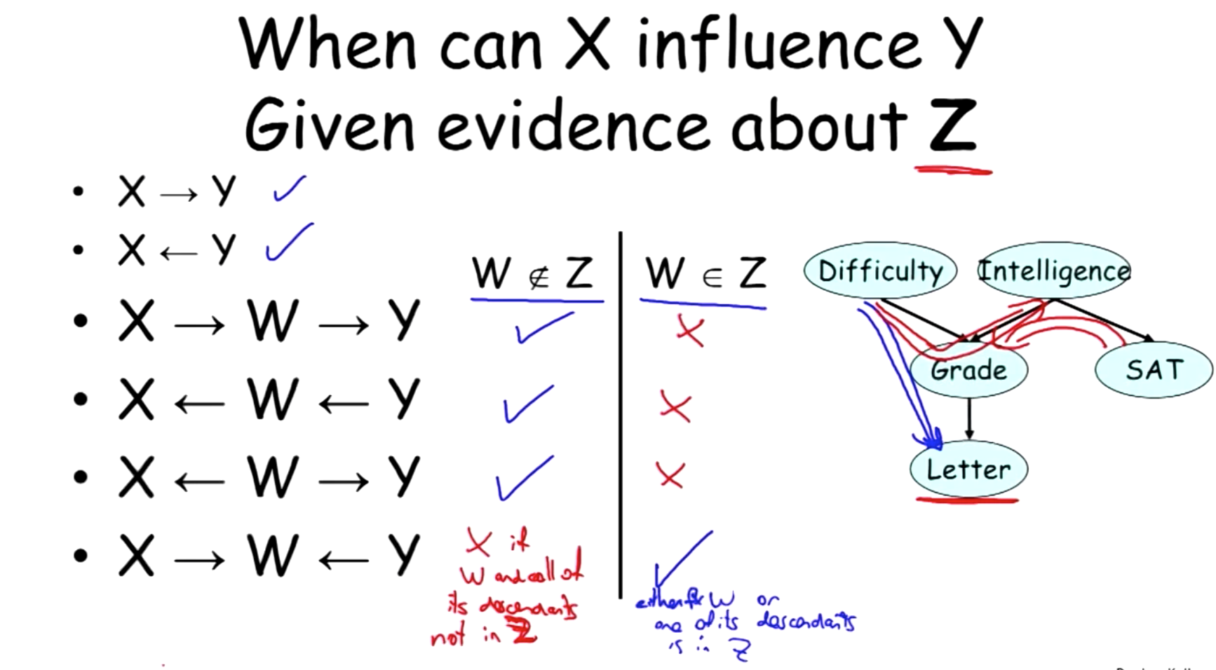
When given evidence about Z, things become more complicate, whether influence can flow depend on whether W is in evidence or not. The most notable stuff is when W or its decendents are in Z, the v-structure actually allows the influence to flow, and otherwise it won’t.
This observation is summarized as the following rule:
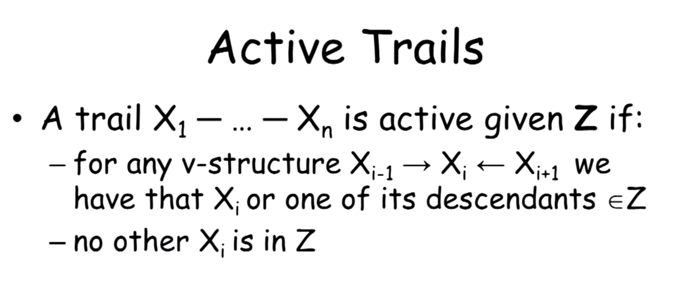
Another way to consider the influence is through independence, so an active trail means \(X_n\) is dependent on \(X_1\),and condition can both gain and lose independence.
Naive Bayes
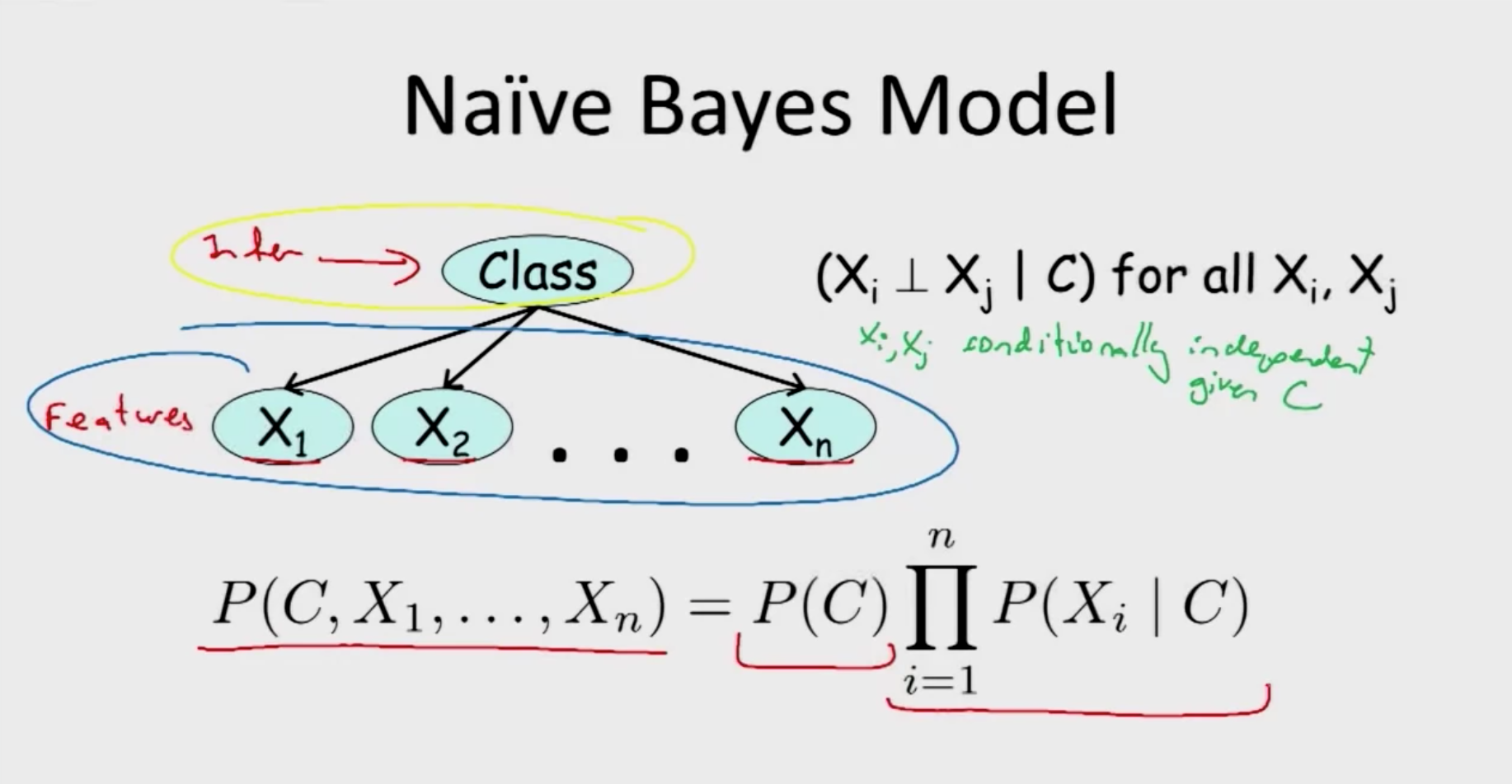
As we can see from the graph model below, Naive Bayes assumes that once class is observed, all the features are independent with each other, which is a quite strong assumption. But with this assumption, we can easily write the joint probability distribution as:
\(P\left(C, X_{1}, \ldots, X_{n}\right)=P(C) \prod_{i=1}^{n} P\left(X_{i} \mid C\right)\)
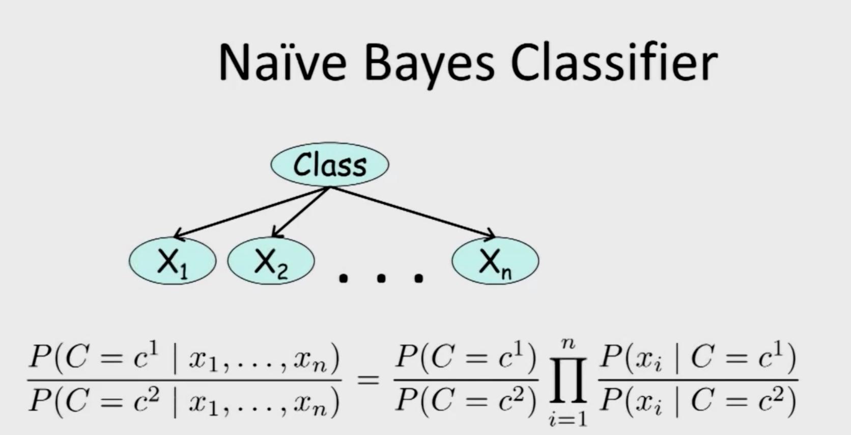
And the direct application of Naive Bayes is Naive Bayes Classifier, which utilizes the strong assumption, given the observed features, we can classify which class this set of observations belongs using bayes theorem.